

Comparison with linear theory#
The figures on this page compare simulations with the roots of the kinetic dispersion
relation for the same populations, computed with the plasma dispersion function in
docs/scripts/dispersion.py. The numbers quoted in the text are read from the same runs
that produced the figures.
Two things decide whether a rate can be measured at all, and both are about the range between the noise floor and saturation rather than about the numerical scheme. A mode that emerges from the particle noise and saturates two e-foldings later cannot be fitted however carefully the window is chosen; loading the plasma quietly and seeding one mode opens that range to five or more e-foldings. And the window itself has to be chosen by a rule rather than by eye, because a short window sitting on a noise excursion will happily return any rate at all.
The rule used here, implemented as robust_growth_fit in docs/scripts/common.py, is to
keep the longest window inside the growth phase whose straight-line fit to
\( \ln(\text{mode energy}) \) reaches a coefficient of determination of 0.95, subject to
the window spanning at least 15 \( \omega_{pe}^{-1} \) and 1.5 e-foldings. A mode for which
no window qualifies is reported as such and left out of the comparison, rather than
fitted over a window picked to make it agree. That is why some modes are missing from
the panels below.
Landau damping#
A quiet start (equally spaced positions, Maxwellian velocities at the quantiles of a
bit-reversed sequence, supplied through initial_positions and initial_velocities)
with 300000 electrons, a displacement perturbation of relative
amplitude \(ak = \) 0.01 and \(k\lambda_D = \) 0.501.

(a) Electrostatic energy with the fit through its maxima, \(\gamma = \) -0.144 \(\,\omega_{pe}\),
and the kinetic root \(\gamma = \) -0.154 \(\,\omega_{pe}\). (b) The first
Fourier mode of \(E_x\) with the theoretical envelope; the frequency from the zero
crossings is \(\omega_r = \) 1.4 \(\,\omega_{pe}\) against
1.42 \(\,\omega_{pe}\). The wave decays through
5.51 e-foldings before reaching the noise floor. Generated by
docs/scripts/fig_landau_damping.py.#
The quiet start matters: with random velocities and 40000 particles the noise floor
is reached after one e-folding, and with the large amplitude of
examples/Landau_damping.py the wave is in the trapping regime and damps faster than
the linear rate (see Landau damping).
Two-stream instability#
The configuration of examples/input.toml with 14000
particles per species (four times the file’s value). The first mode of the box has
\(k\lambda_D = \) 0.179 and \(kv_d/\omega_{pe} = \) 1.01;
the kinetic root is a purely growing mode with
\(\gamma = \) 0.106 \(\,\omega_{pe}\).
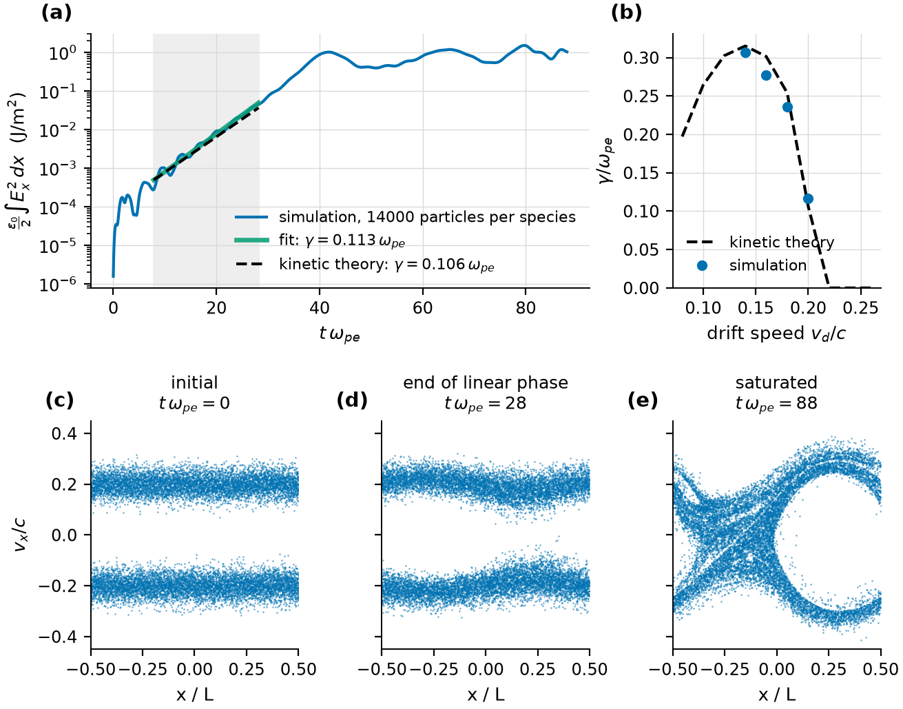
(a) Electrostatic energy; the rate fitted in the shaded window, chosen from the
first Fourier mode between thirty times its initial level and three percent of its
peak, is \(\gamma = \) 0.113 \(\,\omega_{pe}\). (b) Growth
rate of the first mode against the drift speed, from ten runs of the same compiled
program with the drift passed as a runtime input; the mean deviation from theory over
the usable points is 0.0686. (c-e) Electron
phase space. Generated by docs/scripts/fig_two_stream.py.#
Near the cold-beam threshold \(kv_d = \omega_{pe}\) the growth rate is sensitive to the thermal spread and the linear phase is short, because the instability starts from the noise of the particle sampling and saturates after a few e-foldings. The rates fitted from runs with the 3500 particles of the input file scatter by tens of percent around the kinetic value; the scan in panel (b) shows the agreement that the larger particle number gives.
Bump-on-tail instability#
A weak electron beam on the tail of a Maxwellian drives Langmuir waves through inverse
Landau damping. Run as examples/bump-on-tail.toml is written, every mode emerges from
the particle-noise floor and the fastest saturates about two e-foldings later, so there
is no exponential phase to fit. The run below reloads the same four populations with a
quiet start, and displaces the bulk electrons at the wavenumber of the fastest-growing
mode, mode 7 of the box. That drops the noise floor far enough for
the mode to grow through 5.36 e-foldings before it saturates.

Quiet start with 12000 pseudo-particles per population and a
seed of relative amplitude \( ak = \) 0.001 on mode
7 (\( kc/\omega_{pe} = \) 4.9); the beam
carries 3 % of the bulk density. (a) Electron velocity
distribution at the start and at the end: the beam has flattened into a plateau.
(b) Amplitude of the seeded mode. The fit over
[0, 75.2] \( \omega_{pe}^{-1} \) gives
\( \gamma = \) 0.0713 \( \,\omega_{pe} \) against
0.0808 \( \,\omega_{pe} \) from the kinetic dispersion relation,
low by 11.7 %. The measured real frequency is
0.986 \( \,\omega_{pe} \) against
0.99 \( \,\omega_{pe} \), a difference of
0.407 %. (c) Electron phase space at the end of the
linear phase, showing the 7 holes of the seeded mode. (d) The
saturated state. Generated by docs/scripts/fig_bump_on_tail.py.#
Only the fastest mode is quoted. Seeding a slower mode in the same box does not isolate it: mode 7 still grows out of the residual noise and saturates the plasma first, which cuts the slower mode’s growth short and biases its fitted rate low, by ten to forty percent for the modes on either side of the peak. Those points are left out rather than shown as a comparison. Measuring them properly needs a box holding a single wavelength, one run per wavenumber, which is what the Weibel case below does.
Weibel instability#
The electrons carry the temperature anisotropy of examples/Weibel_instability.py,
\( T_z/T_x = \) 100, which drives a purely growing transverse mode.
One simulation is run per wavenumber. Each starts quiet and adds a small modulation
\( v_z \to v_z + \delta \sin(kx) \) to the electrons, whose current seeds \( B_y \) at that
one wavenumber; started from particle noise instead, the modes rise only about two
e-foldings above the floor and no rate can be fitted.

8000 pseudo-particles per species on 150 cells,
1800 steps at \( c\,\Delta t/\Delta x = \) 0.5, seed
amplitude 0.001 of the thermal speed, filter off. (a) \( B_y(x, t) \) for the
seeded fastest mode. (b) Amplitude of three seeded modes with the fitted windows; the
first few inverse plasma times are the seed settling onto the growing eigenmode.
(c) Growth rate against the transverse dispersion relation, for the
5 of 10 modes whose fit met the criterion
below; the mean deviation is 6.3 % and the largest is
11.1 %. The total energy changes by
7.88e-05 over the run. Generated by docs/scripts/fig_weibel.py.#
The modes that are not plotted are those for which no window satisfied the criterion, either because the seed had not separated from the noise or because the mode was still settling when saturation began. They are dropped rather than fitted over a window chosen by hand.
Energy conservation#

examples/input.toml with the explicit and the implicit integrator. (a) Electrostatic
energy. (b) Relative change of the total energy: 0.00321 at
most for the explicit scheme, 2.12e-13 for the implicit one.
Generated by docs/scripts/fig_energy_conservation.py.#
Reproducing these results#
pip install scipy
python docs/scripts/make_all.py
regenerates every figure and docs/_static/figures/measurements.json. Each script is
self-contained and documents the parameters that differ from the corresponding example.